Subscribe for New Post Notifications

Let's look at some Excel VLookup function examples and explore how to use the VLookup function as a worksheet function in Microsoft Excel:

VLOOKUP function in Microsoft Excel

Summary

The VLOOKUP function searching for a value in the first column of a table and retrieve the value in the same row in the index_num position. VLOOKUP supports approximate and exact matching, and wildcards (* ?) for partial matches. VLOOKUP function performs a vertical lookup. Lookup values must appear in the first column of the table, with lookup columns to the right.
The SUBSTITUTE function is a built-in function in Excel that is categorized as a Lookup & Reference Function.

What Does It Do?

It searches for the value you specify and returns a matching value from another column.

Return value

The matched value from a table.

Syntax

=VLOOKUP (lookup_value, table_array, col_index_num, [range_lookup])

Parameters or Arguments

lookup_value - The value to search for in the first column of a table.
table_array - The range of data from which to retrieve a value.
col_index_num - The column number in the table from which to retrieve a value. The first column is 1.
range_lookup - [optional] Enter FALSE to find an exact match. Enter TRUE to find an approximate match (default).

Formatting

No special formatting is needed.

Usage notes

  • Set range_lookup to (FALSE or 0) to require an exact match and (TRUE or 1) to allow a non-exact match.
  • If you specify FALSE in range_lookup parameter and no exact match is found, then the vlookup function will return #N/A error.
  • If you specify TRUE in range_lookup parameter and no exact match is found, then the next smaller value is returned.
  • If range_lookup parameter is TRUE make sure that lookup values in the first row of the table are sorted in ascending order (top to bottom). else, vlookup may return an incorrect or unexpected value.
  • If range_lookup parameter is FALSE, values in the first column of table do not need to be sorted.
  • If col_index_num is less than 1, the vlookup function will return #VALUE! error. In case is greater than the number of columns in table, the vlookup function will return #REF! error.
  • If you have data organized horizontally, use the HLOOKUP function.
  • Do you want to look up a value based on multiple criteria? Use the INDEX and the MATCH function.
  • Excel VLOOKUP is case-insensitive, meaning that uppercase and lowercase characters are treated as equivalent.
  • Always use absolute cell references (with the $ sign) for the table_array argument to prevent it from changing when copying your formula to other cells.

Example

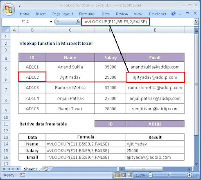
How to use VLOOKUP function in Microsoft Excel.

VLOOKUP function in Microsoft Excel

First Parameter
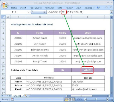
The first parameter is the value to search for in the table of data.

VLOOKUP function in Microsoft Excel

In this example, the first parameter is AD102. This is the value that the VLOOKUP will search for in the first column of the table of data.

Second Parameter
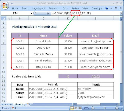
The second parameter is the table or the source of data where the vertical lookup should be performed.

VLOOKUP function in Microsoft Excel

In this example, the second parameter is B5:E9 which gives us to data to use in the vertical lookup.

Third Parameter
The third parameter is the position number in the table where the return data can be found.

VLOOKUP function in Microsoft Excel

In this example, the third parameter is 2. This means that the second column in the table is where we will find the value to return.

Fourth Parameter
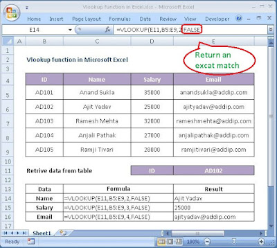
The fourth parameter determines whether you are looking for an exact match or approximate match.

VLOOKUP function in Microsoft Excel

In this example, the fourth parameter is FALSE. A parameter of FALSE means VLOOKUP function is looking for an EXACT match for the value of AD102. A parameter of TRUE means that a close match will be returned.

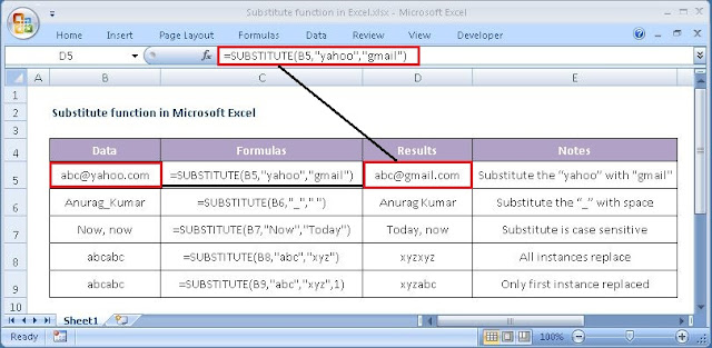
Let's look at some Excel Substitute function examples and explore how to use the Substitute function as a worksheet function in Microsoft Excel:

SUBSTITUTE function

Summary

The SUBSTITUTE function is as similar to the REPLACE function used in the excel. However, SUBSTITUTE function replaces one or more instances of a substituted text string with a specified character(s). Whereas REPLACE function only replaces the text in a specified position/location of a supplied string.
Substitute function can be useful for when you want to substitute old text with a new text in the given text. For example, if the given text is 9988-776-655 and you want it as 9988776655 then you can use SUBSTITUTE function to transform this.
The SUBSTITUTE function is a built-in function in Excel that is categorized as a Text Function.

What Does It Do?

Replace text based on content.

Return value

The string/text Value.

Syntax

=SUBSTITUTE (text, old_text, new_text, [instance_num])

Parameters or Arguments

text - The original string to use to perform the substitution.
old_text - The text to replace.
new_text - The new text to replace with.
instance_num - The instance to replace. If omitted, every occurrence of the old text will be changed to the new text.

Formatting

No special formatting is needed.

Substitute different characters with a single formula

You can nest several SUBSTITUTE functions within a single formula to do several substitutions at a time, i.e. substitute multiple characters with a single formula.

Below are the example of this.

Nested Substitute

Usage notes

  • The Excel Substitute function can replace text by matching. Use the Substitute function when you want to replace text based on its content, not position. Optionally, you can specify the instance of found text to replace (i.e. first instance, second instance, etc.).
  • Substitute function finds and replaces old_text with new_text in a text string.
  • If you specify an instance number, then only that instance of the old text is replaced. Otherwise, every occurrence of old text in the text string is changed to new text.
  • Use SUBSTITUTE function to replace text based on content. Use the REPLACE function to replace text based on its location.
  • Substitute function is case-sensitive.
  • Substitute function does not support wildcards.

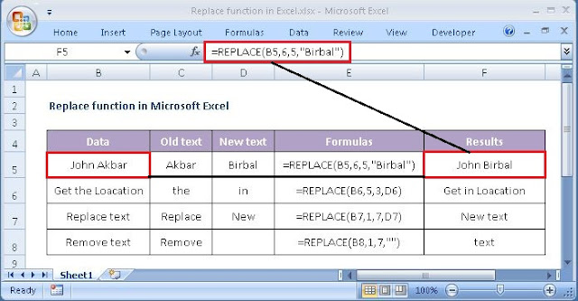
Let's look at some Excel Replace function examples and explore how to use the Replace function as a worksheet function in Microsoft Excel:

REPLACE function in Microsoft Excel

Summary

The Excel REPLACE function replaces characters specified by position in a given text string with another text string.
The REPLACE function is a built-in function in Excel that is categorized as a Text Function.

What Does It Do?

Replaces a portion of text with a new piece of text.

Return value

The altered text.

Syntax

=REPLACE (old_text, start_num, num_chars, new_text)

Parameters or Arguments

old_text - The original string value.
start_num - The starting position in the text to replace.
num_chars - The number of characters to replace in old_text.
new_text - The text to replace old_text with.

Formatting

No special formatting is needed.

Usage notes

The REPLACE function is useful for replacing text at a known position in a given string. For example, the following formula replaces 4 characters starting at the 1st character:

=REPLACE("Tech World",1,4,"Information")//
returns "Information World"

  • #NAME? - Occurs if text data entered as the Old_text argument is not enclosed in double quotation marks - row five above.
  • #VALUE! - Occurs if the Start_num or Num_chars arguments are negative or contain non-numeric values - row eight above.
  • Use the REPLACE function when you want to replace text based on a known location.
  • Use FIND or SEARCH to find and replace text when the location is not known in advance.
  • Use SUBSTITUTE to replace one or more instances of text based on content only.

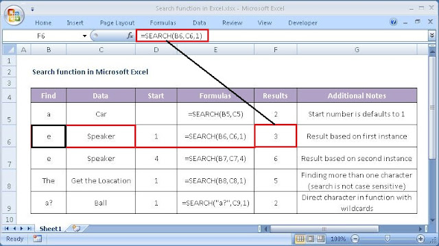
Let's look at some Excel Search function examples and explore how to use the Search function as a worksheet function in Microsoft Excel:

SEARCH function

Summary

The SEARCH function is a way to find a character or string within another cell, and it will return the value associated with the starting place. In other words, if you are trying to figure out where a character is within the cell that contains a word, sentence or other type of information, you could use the SEARCH function.
SEARCH returns the position of the first character of find_text inside within_text. Unlike FIND, SEARCH allows wildcards, and is not case-sensitive.
The SEARCH function is a built-in function in Excel that is categorized as a Text Function.

What Does It Do ?

Get the location of text in a string.

Return value

A number representing the location of find_text.

Syntax

=SEARCH(find_text, within_text, [start_num])

Parameters or Arguments

find_text - The text to find.
within_text - The text to search within.
start_num - Starting position in the text to search. Optional, defaults to 1.

Formatting

No special formatting is needed, the result will be shown as a number.

Usage notes

  • Use the SEARCH function to get the location of one text string inside another.
  • SEARCH returns the position of the first character of find_text inside within_text.
  • SEARCH function is not case-sensitive, the upper-case and lower-case find_text values, "M" and "m", return the same result.
  • SEARCH function allows using the wildcard characters.
  • SEARCH allows the wildcard characters question mark (?) and asterisk (*), in find_text.
  • The ? matches any single character and the * matches any sequence of characters. To find a literal ? or *, use a tilde (~) before the character, i.e. ~* and ~?.
  • If the SEARCH function does not find a match, it will return a #VALUE! error.

Let's look at some Excel Find function examples and explore how to use the Find function as a worksheet function in Microsoft Excel:

FIND function

Summary

The FIND function in Excel is used to return the position of a specific character or sub-string within a text string.
The FIND function is a built-in function in Excel that is categorized as a Text Function.

What Does It Do ?

Get the location of text in a string.

Return value

A number representing the location of find_text.

Syntax

=FIND(find_text, within_text, [start_num])

Parameters or Arguments

find_text - The text to find.
within_text - The text to search within.
start_num - The starting position in the text to search. Optional, defaults to 1.

Formatting

No special formatting is needed, the result will be shown as a number.

Usage notes

  • If the find_text argument contains several characters, the FIND function returns the position of the first character. For example, the formula FIND("en","sentence") returns 2 because "e" in the 2nd letter in the word "sentence".
  • If within_text contains several occurrences of find_text, the first occurrence is returned. For example, FIND("l", "Ball") returns 3, which is the position of the first "l" character in the word "Ball".
  • If find_text is an empty string "", the Excel FIND formula returns the first character in the search string.
  • The location is returned as the number of characters from the start of within_text.
  • Start_num is optional and defaults to 1.
  • The Excel FIND function returns the #VALUE! error if any of the following occurs:
  • =>Find_text does not exist in within_text.
    =>Start_num contains more characters than within_text.
    =>Start_num is 0 (zero) or a negative number.
  • The FIND function is case sensitive and does not allow wildcard characters.
  • If you are looking for a case-insensitive match, use the SEARCH function and/or to use wildcards.

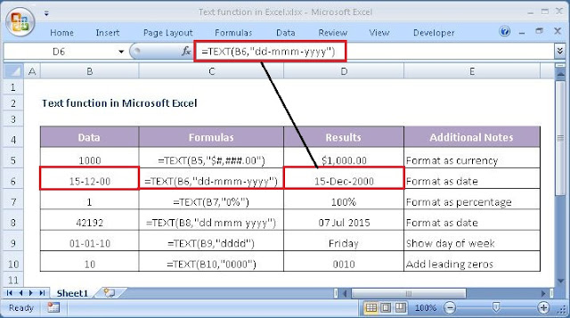
Let's look at some Excel Text function examples and explore how to use the Text function as a worksheet function in Microsoft Excel:

TEXT function

Summary

Text function in excel is basically used to convert the numeric values into a text format that is specified. So, it takes a value and turns it into text based on the numeric format of your choice.
The Text function is a built-in function in Excel that is categorized as a Text Function.

What Does It Do ?

This function converts a number to a piece of text. The formatting for the text needs to be specified in the function.

Return value

A number as text in the given format.

Syntax

=TEXT(value, format_text)

Parameters or Arguments

value - The numerical value that we need to convert to text. format_text - The format we want to apply.

Formatting

No special formatting is required.

When is the Excel TEXT Function required?

  1. We want to display dates in a specified format.
  2. We wish to display numbers in a specified format or in a more legible way.
  3. We wish to combine numbers with text or characters.

Usage notes

  • Use the TEXT function to convert a number to text in a specific number format.
  • The data converted into text cannot be used for calculations. If needed, we should keep the original data in a hidden format and use it for other formulas.
  • TEXT is especially useful when you want to embed the numeric output of a formula or function and present it in a particular format inside other text. For example, "Sales last year increased by over $10,500", where the number 42100 has been formatted with a currency symbol and thousands separator.
  • The TEXT function returns the #NAME? error if you omit the quotation marks around the format code. For example the formula =TEXT(A2, mm/dd/yy) is incorrect and should be written this way: =TEXT(A2, "mm/dd/yy").
  • The TEXT function in Excel is language-specific, and requires using region-specific date and time format codes.
  • format_text must appear in double quotation marks.

Let's look at some Excel Rept function examples and explore how to use the Rept function as a worksheet function in Microsoft Excel:

REPT function

Summary

The Microsoft Excel REPT function returns a repeated text value a specified number of times. For example, =REPT("ABC",3) returns "ABCABCABC".
In financial analysis, This can be useful if you want to fill a cell, or pad values to a certain length. We can also build histograms, a chart commonly used in financial modeling, using the function by translating values directly into a certain number of (repeated) characters.
The Rept function is a built-in function in Excel that is categorized as a Text Function.

What Does It Do ?

Repeats a piece of text a specified number of times.

Return value

The repeated text.

Syntax

=REPT (text, number_times)

Parameters or Arguments

text - The text value to repeat.
number_times - It is the positive number that specifies the number of times to repeat text.

Formatting

No special formatting is needed.

Usage notes

  • The number_times parameter of the REPT function must be a positive number.
  • The result of the REPT function cannot be longer than 32,767 characters, or else it will return a #VALUE! error.
  • If number_times is not an integer, it is truncated. For example, if you use the number 10.8, it will only consider 10 and repeat the specified text 10 number of times.
  • If number_times is 0 (zero), REPT returns “” (empty text).

The REPT function repeats characters a specified number of times. For example, to repeat "A" six times, you can use the following formula:

=REPT("A",6) // returns "AAAAAA"

Inputs to REPT can be variable. In the example shown, REPT is configured to repeat the string in column B using the count in column C. The formula in D5 is:

=REPT(B5,C5) // returns "@@@@@"